Q-Meter Circuit Simulator
The electronic response of a series-tank Q-meter, as used for cw-NMR polarization measurements on polarized targets. An RF sweep drives a tuned LCR tank through a constant-current resistor; the signal is read as a diode (magnitude) output and as a phase-sensitive mixer output against a reference line. Supply, signal, reference and coil (λ/2) cables are all modeled as lossy transmission lines. Based on the MathCAD model of Court, Houlden et al., computed live in your browser with Python.
Cable lengths
Each transmission line length in units of λ/2 at the Larmor frequency. The coil (λ/2) cable sits in the tank between the tuning capacitor and the coil, and has the largest effect on the curve shape.
Diode signal
Phase signal
Analyzing the signal
How it works from raw sweep to polarization, step by step
A Q-meter sweep becomes a polarization in a few steps, as in NMR_Analysis and rgc_offline. Here they run on the simulated phase signal at the polarization set above, with a thermal-equilibrium (TE) signal from the same circuit as the calibration. Because the true polarization is known, you can see how well each method recovers it.
- Baseline subtraction. A baseline sweep, taken with the NMR line moved out of the window by shifting the field, is subtracted. Here the baseline is the same circuit with no signal. If the circuit drifts between the two sweeps (cable temperature, tune), a background remains; the drift control changes the tuning capacitance of the signal sweeps to mimic this.
- Polynomial fit. A polynomial, usually cubic, is fit to the wings (the sweep away from the line, shaded blue) and subtracted.
- Integration. The fit-subtracted points in the integration range (shaded copper) are summed to give the area .
- Calibration. At thermal equilibrium the polarization is known from the field and temperature, for protons and for deuterons, with . Then and . This assumes the Q-meter responds linearly. Large signals are compressed, which shows up as an error at high proton polarization.
- Deuterons. The asymmetry of the Pake doublet measures the polarization without a TE: the two transitions' intensities are in the ratio and . The quick estimate takes , the ratio of the two peak heights. Each peak sits on the other transition's plateau, which slopes up toward the line center. So a straight line is drawn along the plateau on the step just outside each peak and carried in under the peak, and the height is measured from that line (plot 3). Without this subtraction the ratio is pulled toward 1. For a narrow line this comes within about 1% (absolute) of the true polarization, but it over-reads as the line broadens and the peaks' tails lean on the plateau. Where the step and the peak merge, no pedestal can be found and the raw heights are used. A fit of the full lineshape, as in DeuteronPeakFit, does better, but only if the output is pure absorption: cables rotate the signal's phase and mix in dispersion. The complex fit adds a phase angle to absorb this. Try both before and after pressing the phase plot's Tune button.
1. Raw sweep and baseline
2. Baseline subtracted, with polynomial
3. Fit subtracted, integrated
4–5. Polarization
Circuit constants fixed values from the notebook and the deuteron lineshape; change with care
The circuit schematic and the model, equation by equation
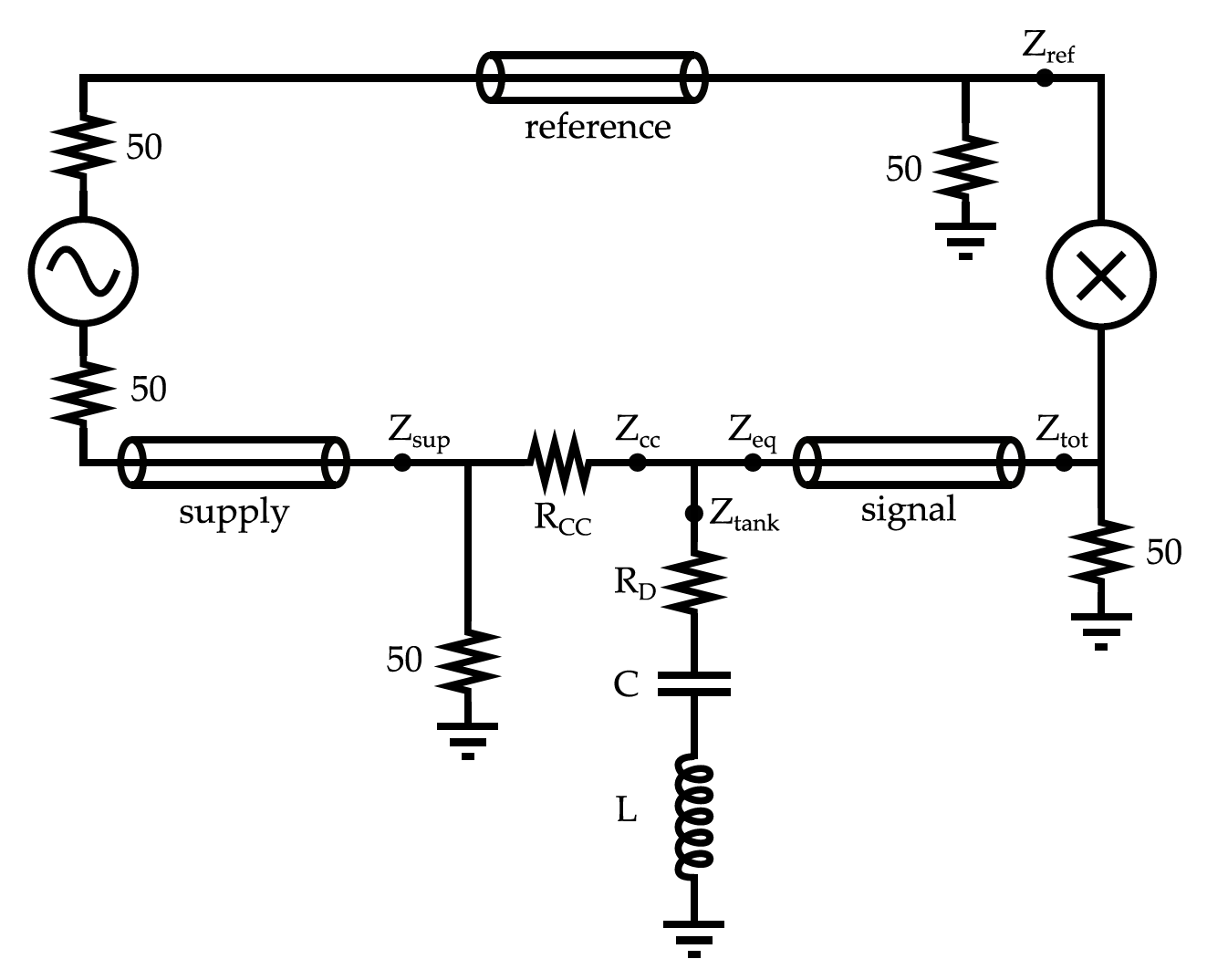
- An RF source drives the tank through a supply line and a constant-current resistor Rcc; a reference line carries the source directly to the mixer.
- The series tank (damping R, tuning C, coil L) has a fourth transmission line between C and L, usually called the λ/2 cable. The signal line connects the tank to the other side of the mixer.
- Capacitance is in units of the value that tunes the bare tank (no cables) to the Larmor frequency for the chosen species at 5 T. Phase is in degrees from ideal tune with zero line length.
- The optional polarization signal enters as a complex susceptibility multiplying the coil inductance, L = L0(1 + 4πηχ). For protons the lineshape is fitted to measured signals at polarizations from 24% to 79%, so it shifts and sharpens as the polarization grows; its size follows Seely's susceptibility and Hill & Hill's normalization. For deuterons it is the Pake doublet of Dulya et al., ported from DeuteronPeakFit, with its dispersion as well as its absorption.
- Polarization has its physical sign: positive is absorptive, as at thermal equilibrium. The
notebook's
polis the negative of this, so its default of −0.0027 is +0.27% here. - The supply, signal and reference lines end in 50 Ω, close to the cable's characteristic impedance, so they are matched. Their lengths only delay and attenuate the RF, and don't change the shape of the Q-curve, as in Court et al. The delay rotates the phase signal; a reference cable as long as the supply and signal cables together cancels it, and the phase Tune button corrects it.
- The schematic leaves out the coil cable between C and L.
- Lengths are in units of λ/2, so a coil cable of 1 is a true λ/2 line that passes the coil impedance through almost unchanged. Near 0.5 (λ/4) the line makes the coil look capacitive, and the series tank cannot be tuned.
Every quantity is evaluated at each sweep frequency ω. Lines are labeled i ∈ {sup, sig, ref, coil}, , and is the input impedance of line i terminated by . Each stage is reduced to a Thevenin source (an open-circuit voltage and a source impedance) and carried through the next line.
Larmor frequency and tuning capacitor
The capacitance control is in units of the capacitor that resonates the bare coil at , with and MHz/T, and the field fixed at T (212.88 MHz for protons, 32.68 MHz for deuterons).
Transmission lines
is the cable length control, and , , are the cable's resistance, inductance and capacitance per meter, so whatever the length. A source with impedance at one end of a line gives the open-circuit voltage and source impedance at the other. For a matched line, , these are and : a delay and attenuation only.
Coil
is the filling factor and the complex susceptibility of the polarized sample, given below for protons and deuterons. With the signal off, .
Proton signal
with (Seely). is fitted to measured proton lines from a 5 T target (2022), taken while the polarization was growing: spin-ups from 7% to 78% and the build-up after two reversals from −31% to −73%, with for positive and for negative . Near the line is nearly symmetric and about 46 kHz wide. As grows it moves up, the local field of the polarized sample, and sharpens on the high-frequency side, to 37 kHz wide with a long low-frequency tail at 78%. For negative it moves down and sharpens on the low-frequency side, nearly the mirror image with a longer tail: 44 kHz wide at −73%. Beyond the measured range the shape is held and only the shift and size follow . A real line also depends on how fast the polarization is changing, which this model leaves out. , so the area does not depend on . Between samples and are straight lines, sums of triangles , whose Hilbert transforms are exact, so is the exact Kramers–Kronig partner of . The area is that of Hill & Hill's line (more on the proton line).
Deuteron signal
and are the powder-averaged absorption and dispersion integrals of Dulya et al., with broadening and EFG asymmetry ; the full include a small dependence. scales Seely's proton value by the spin-1 magnetization at the same density. is the Hilbert transform, which makes the Kramers–Kronig partner of .
Tank, supply and signal line
is the damping resistor, the source impedance, and the 50 Ω is the supply line's termination to ground. , , and are the source impedances looking back toward the RF source.
Voltages at the mixer
The mixer inputs are terminated by (the 50 Ω at each mixer input in the schematic). The mixer responds to the phase difference between its inputs, hence , so the reference cable's delay offsets the supply and signal cables' delay.
The Tune buttons
Both use the baseline (signal off) and leave cable lengths alone. Diode tune scans for the dip and refines it by bisection. Phase tune first does the diode tune. Both roots make the phase output an extremum at ; it picks the one for which an absorptive signal points the same way as in the ideal zero-length circuit. When the reference cable's delay doesn't match the supply and signal cables', the baseline at that phase can be a dip rather than a peak.
References
- J.D. Maxwell, J. Brock, C. Cuevas, H. Dong, C.D. Keith, J.J. Pierce, “A new cw-NMR Q-meter for dynamically polarized targets for particle physics,” NIM A 1087 (2026) 171417. doi:10.1016/j.nima.2026.171417
- G.R. Court, M.A. Houlden et al., “High precision measurement of the polarization in solid state polarized targets using NMR,” NIM A 527 (2004) 253–263. doi:10.1016/j.nima.2004.02.041
- J.J. Hill, D.A. Hill, “Simple correction for Q-meter measurement of proton target polarization,” NIM 116 (1974) 269–274. doi:10.1016/0029-554X(74)90613-2
- Seely et al., “Simulation and Tuning of the TUNL NMR System,” Proceedings of the Workshop on NMR in Polarized Targets (1998).
- C. Dulya et al., “A line-shape analysis for spin-1 NMR signals,” NIM A 398 (1997) 109–125. doi:10.1016/S0168-9002(97)00317-3
- Yu.F. Kisselev, C.M. Dulya, T.O. Niinikoski, “Measurement of complex RF susceptibility using a series Q-meter,” NIM A 354 (1995) 249–261. doi:10.1016/0168-9002(94)01066-8
- M. McClellan, “Complex deuteron NMR signals,” Eur. Phys. J. A 61, 176 (2025). doi:10.1140/epja/s10050-025-01644-z